Clean Data in Excel with Power Query: A Step-by-Step Guide
Clean messy data once and refresh it forever. A beginner's guide to Excel Power Query: remove duplicates, fix blanks, merge tables and load clean data.
 Joshua AkintayoData analyst & teacher4 October 2026 · 5 min read
Most of a data analyst’s time isn’t spent on charts. It’s spent cleaning data: removing duplicates, fixing blanks, standardising text and combining tables.
You can do all of that with Excel formulas. But every time new data arrives, you have to do it all again.
Power Query fixes that. You clean the data once, Power Query records every step, and next month you just click Refresh. That’s why I tell my students: clean once, refresh forever.
Here’s a full walkthrough from one of my lessons:
What is Power Query?
Power Query is Excel’s built-in tool for ETL:
- Extract: get data from a CSV, an Excel file, a folder of files, or a database
- Transform: clean and reshape it
- Load: send the clean table back into Excel
It’s built into Excel 2016 and later (on the Data tab, under Get & Transform Data), and the same tool powers data preparation in Power BI. Learn it once and you can use it in both.
Step 1: Get your data in (and don’t load it yet)
- Open a blank workbook.
- Go to Data → Get Data → From File → From Text/CSV (or From Workbook for an Excel file).
- Choose your file.
- In the preview window, click Transform Data, not Load.
“Transform Data” opens the Power Query Editor, where the cleaning happens. “Load” dumps the messy data straight into your sheet.
Tip: if you receive a new file every month, use Get Data → From File → From Folder instead. Power Query combines every file in the folder, so when April’s file arrives you drop it into the folder, click Refresh, and April’s data simply appears.
Step 2: Profile your data before you touch it
Go to the View tab and tick:
- Column quality: shows the percentage of valid, error and empty values in each column
- Column distribution: shows how many distinct and unique values each column has
- Column profile: shows detailed statistics for the selected column
Then click the text in the bottom-left corner that says “Column profiling based on top 1000 rows” and switch it to based on entire data set. Otherwise Power Query only checks the first 1,000 rows and can miss problems further down.
Now you know exactly what needs fixing before you start.
Step 3: Fix headers and data types
- Headers: if your column names are sitting in the first row of data, use Home → Use First Row as Headers. Power Query usually does this automatically.
- Data types: click the small ABC or 123 icon on each column header and set the right type: Text, Whole Number, Decimal, or Date.
Wrong data types cause most of the “my formula returns 0” and “my dates show as 1905” problems beginners run into later.
Step 4: Clean the text
Select your text columns, then:
- Transform → Format → Trim removes extra spaces at the start and end (“Lagos “ becomes “Lagos”).
- Transform → Format → Capitalize Each Word makes names consistent (“funke balogun” becomes “Funke Balogun”).
- Replace Values (right-click the column) fixes inconsistent codes, like
F→FemaleandM→Male. Open Advanced options and tick Match entire cell contents, or you’ll turn “Male” into “Femaleale”.
Step 5: Remove duplicates and handle blanks
- Duplicates: select the column that should be unique (like Order ID), then Home → Remove Rows → Remove Duplicates.
- Blanks: right-click the column → Replace Values. Leave “Value to find” empty (or type
nullif the blanks show as null) and replace them with something meaningful, likeUnassignedorUnknown.
Before you fill blanks, think about what they mean. A missing sales rep might be “Unassigned”; a missing state might be worth asking the business about.
Step 6: Combine tables with Merge Queries
Often the data you need is split across two tables. In my class dataset, the sales table has the product name but not the price. The price is in a separate product lookup table.
- Load the lookup table as its own query.
- Select your sales query, then Home → Merge Queries.
- Click the Product column in both tables.
- Choose the Join Kind:
| Join kind | Keeps |
|---|---|
| Left outer | All rows from the first table, plus matching info from the second (the one you’ll use most) |
| Inner | Only rows that match in both tables |
| Full outer | Everything from both tables |
| Left anti | Rows in the first table with no match (great for finding problems) |
- Click the expand icon (↔) on the new column and tick only the columns you need, like Standard Price.
It’s the Power Query version of VLOOKUP, except it never breaks when columns move. (Not sure about VLOOKUP? Read VLOOKUP vs XLOOKUP.)
Step 7: Add the columns you need
- Add Column → Custom Column for calculations, like
Revenue = [Quantity] * [Standard Price]. - Add Column → Conditional Column for IF-style rules without typing a formula, like labelling orders as Low, Mid or High value.
Step 8: Close & Load, then Refresh forever
Click Home → Close & Load To… → Table → New worksheet. Your clean table lands in Excel, ready for PivotTables and dashboards.
Every step you took is saved in Applied Steps on the right of the editor. Made a mistake? Click the ❌ next to that step and it’s undone. Nothing is ever lost.
When new data arrives, go to Data → Refresh All. Power Query repeats every step, and every PivotTable and chart built on that table updates with it.
The mistake almost every beginner makes
Importing the same file again to fix something. I’ve seen workbooks with the same table loaded four times, the file size ballooning and nobody sure which table is the right one.
To change anything, go to Data → Queries & Connections, right-click the query, and choose Edit. Never import it again.
Recap
- Get Data → Transform Data (not Load).
- Profile your data on the entire data set.
- Fix headers and data types.
- Trim, fix capitalisation and replace inconsistent values.
- Remove duplicates and handle blanks thoughtfully.
- Merge queries to combine tables.
- Add custom and conditional columns.
- Close & Load, then Refresh when new data comes in.
Clean once, refresh forever.